Training of MNIST sample classification model and class activation mapping

This tool is a simple application on the MNIST dataset (70,000 images of handwritten digits, from 0 to 9, each with a resolution of 28x28 pixels) which predicts the digit entered in addition to a map of the discriminative region used by a CNN to identify the category.

The main concepts applied in this example have been:

Implementation of custom loss functions.
Obtaining Class Activation Map of each prediction.

Both concepts are briefly explained below along with code examples.

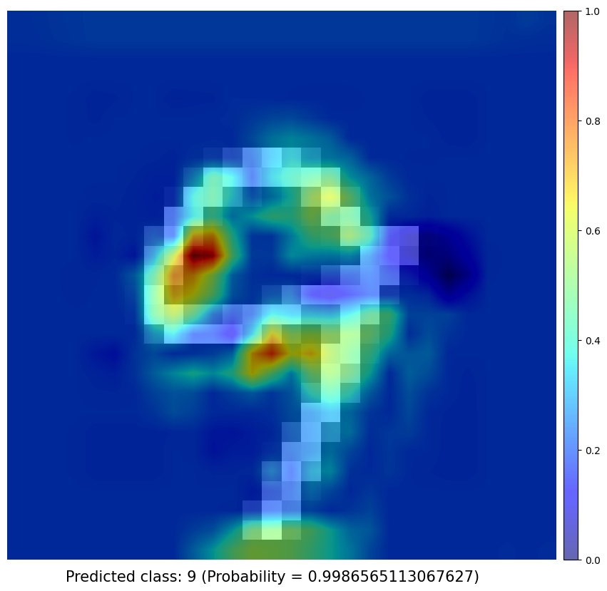
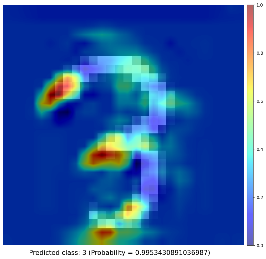
Test samples

Drag and drop an image file.

Implementation of custom loss function

A typical approach for this task is to use a multi-class logistic regression model. This type of network contains a final softmax function which maps the output of the model to a probability distribution over the 10 classes. The cross-entropy loss is commonly used as the loss function for this type of model. The cross-entropy loss calculates the difference between the predicted probability distribution and the actual probability distribution. This probability distribution is given in the form of a one-hot vector in which the sum of all probabilities is 1, with the highest value being the most probable class.

The cross entropy loss is defined as:

\[ L = - \sum_{}{} (y_{i} * log(p_{i})) \]

where \(y_{i}\) is the actual probability of class i and \(p_{i}\) is the predicted probability of class i.

6 iterations of 15 epochs were used, where in each one of them the digits whose number of misclassified samples were above the mean of the total of all the categories are much higher than the other digits. Here is the example of the custom loss function for the MNIST classification task:

                                
                                  class CustomLoss(nn.Module):
                                    def __init__(self, worst_classes_l):
                                        super(CustomLoss, self).__init__()
                                        self.worst_classes = worst_classes_l

                                    def forward(self, output, target):
                                        criterion = nn.CrossEntropyLoss()
                                        loss = criterion(output, target)
                                        mask = torch.Tensor([False]*target.shape[0]).to("cuda")
                                        for i in range(mask.shape[0]):
                                            if target[i] in self.worst_classes:
                                                mask[i] = True
                                        high_cost = (loss * mask.float()).mean()
                                        return loss + high_cost

Comparison of validation accuracy between a model with custom loss function and a model with constant loss function (Using the same training hyperparameters)

Best Validation Accuracy
Model with Custom loss (6 iterations of 15 epochs)	Model with classic Cross Entropy loss function (1 iteration of 90 epochs)
0.98060	0.97580

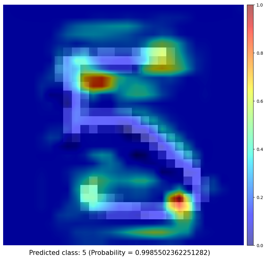
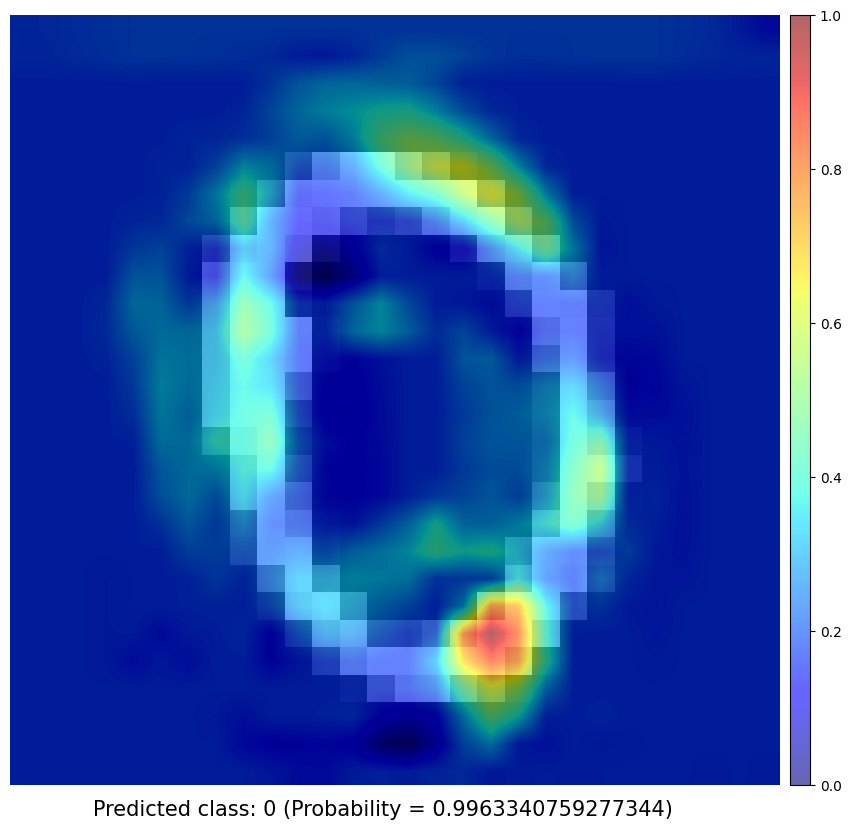
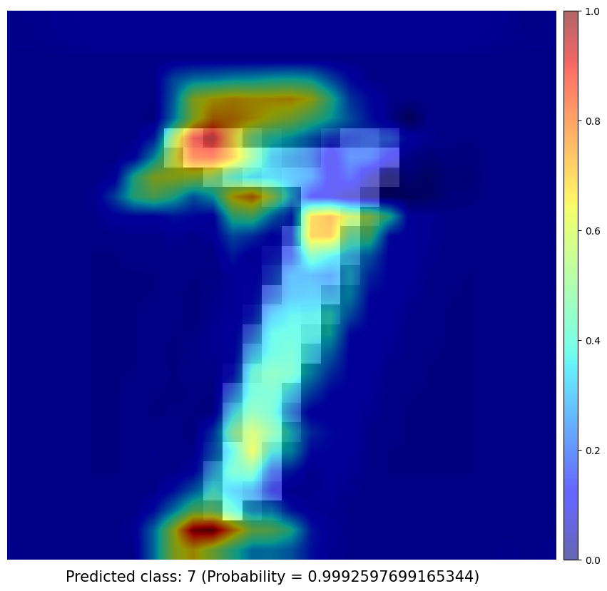
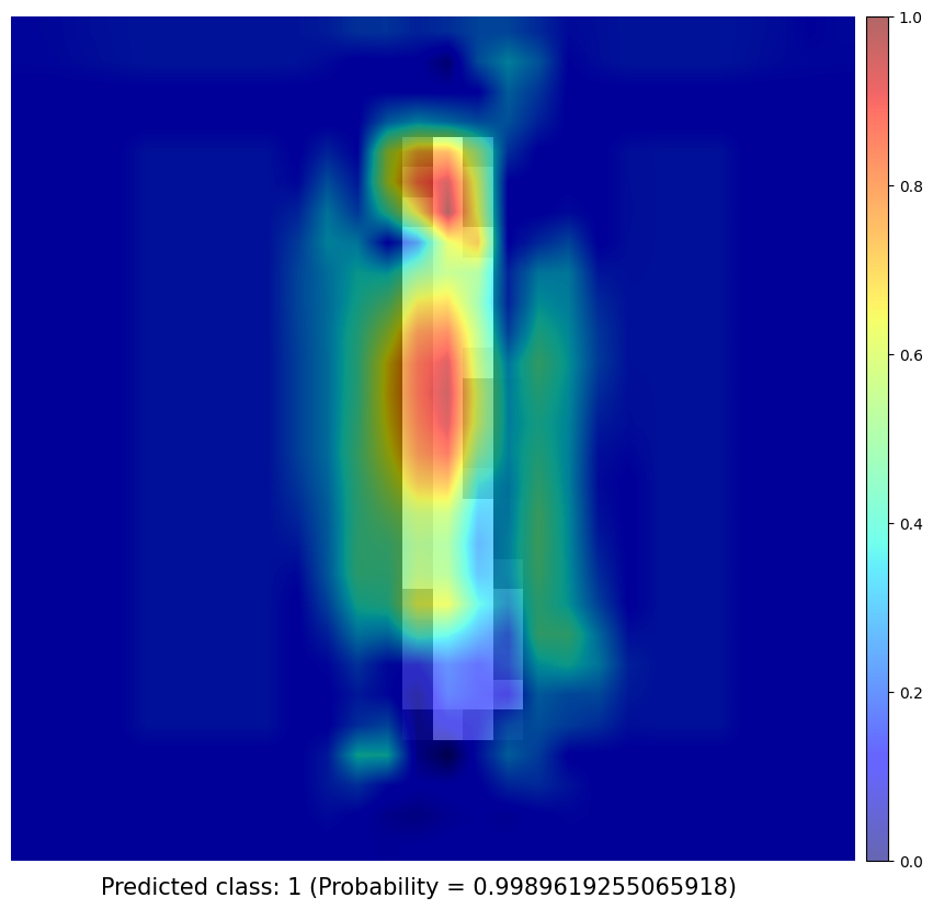
Obtaining Class Activation Map of each prediction

With the increasing performance of Machine Learning, and more specifically with Deep Learning systems and algorithms, the interpretability of developed solutions are gradually decreasing, handling millions of parameters and layers but becoming like black boxes that take the users input and giving beyond expectation outputs but offering no intuition about the causal-effect information that led to such output.

Previous works has shown that the convolutional units of various layers of convolutional networks (CNNs) actually behave as object detectors despite no supervision on the location of the object was provided. Despite having this remarkable ability to localize objects in the convolutional layers, this ability is lost when fully-connected layers are used for classification.

I use a simple network architecture consisting of two convolutional layers and just before the final output layer (softmax in the case of categorization), I perform a global average pooling on the convolutional feature maps and use those as features for a fully-connected layer that produces the desired output. Given this simple connectivity structure, we can identify the importance of the image regions by projecting back the weights of the output layer on to the convolutional feature maps, calling this technique, as already mentioned, as class activation mapping. A more in-depth explanation can be found in the paper.

Model summary

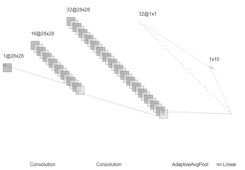
The outputs obtained with the original approach were satisfactory but it was still confusing because it wasn’t completely clear due to loss of spatial information by the subsequent max-pooling layers after each convolutional layer, as a classic layer architecture in this type of problem.